Phenotype prediction

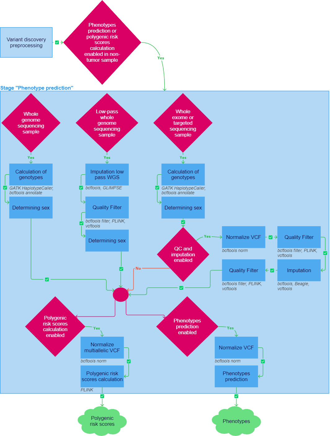
After the "Variant discovery preprocessing" stage has been successfully completed, the phenotype prediction pipeline can be launched for non-tumor samples if at least one of the following tasks was included in the analysis workflow: "Phenotypes prediction" or "Polygenic risk scores calculation".

If any of the following tasks fail, the sample analysis stops. However, if quality control and imputation are included in the analysis workflow, and if the sample does not meet the quality control criteria, the "Phenotype prediction" stage interrupts, but the sample analysis can proceed with report generation.

Convert BAM to VCF#

To move on to phenotypes prediction or polygenic risk scores calculation, it is necessary to generate a VCF file with germline variants that satisfy certain conditions from a sample alignment file in BAM format. The way of preprocessing differs for samples with different sequencing types.

Preprocessing of whole genome sequencing sample#

If the sample sequencing type is defined as "WGS" (whole-genome sequencing), the alignment file is converted to a VCF file during the "Calculation of genotypes" task.

Calculation of genotypes#

GATK HaplotypeCaller produces calls at germline variant sites and confident reference sites, that are needed to calculate the polygenic risk scores of phenotypes, in an alignment file. The calling is accomplished via local de novo assembly of haplotypes in an active region. In other words, whenever the program encounters a region showing signs of variation, it discards the existing mapping information and completely reassembles the reads in that region. This allows to be more accurate when calling regions that are traditionally difficult to call, for example when they contain different types of variants close to each other. For each potentially variant site, the program applies Bayes' rule, using the likelihoods of alleles given the read data to calculate the likelihoods of each genotype per sample given the read data observed for the sample. The most likely genotype is then assigned to the sample.

The variants are then annotated with rsIds from the dbSNP database using bcftools annotate. The resulting file is compressed into a GZIP archive using bgzip. It can be downloaded in the "Result files" section in the "Calculation of genotypes" task details ("Download VCF_GZ"). In addition, the file is indexed using tabix. The resulting index file can be downloaded in the same section ("Download VCF_TBI").

Preprocessing of low-pass whole genome sequencing sample#

If the sample sequencing type is defined as "Low-pass WGS" (whole genome sequencing with low coverage), the alignment file is converted to a VCF file during the "Imputation low pass WGS" task, followed by the mandatory "Quality Filter" task (described below).

caution

The pipeline for phenotypes prediction and polygenic risk scores calculation in low-pass WGS data is experimental.

Imputation low pass WGS#

Imputation is a statistical method for reconstructing missing genetic data based on haplotype analysis in a reference set. First, genotype calling for low-coverage data is performed using bcftools mpileup and bcftools call. As a result, VCF file containing genotype likelihoods (GLs) for each site from the reference panel is generated. This file is then taken as input by the GLIMPSE tool. In addition, variants are divided by chromosomes for parallel imputation. Then, GLIMPSE chunk creates imputation chunks from data to make the calculation more optimized and phases common sites. GLIMPSE phase imputes and phases low-coverage sequencing data. As a reference, the panel based on the 1000 Genomes Project sample collection to 30x coverage is used. GLIMPSE ligate phases rare variants onto a scaffold of common variants, and ligates all phased chunks into a single whole chromosome file. Finally, the imputed variants, divided by chromosomes, are concatenated into a single VCF file using bcftools concat. This file is then sorted by chromosome and compressed into a GZIP archive using bgzip. The resulting file with imputed variants in VCF format can be downloaded in the "Result files" section in the "Imputation low pass WGS" task details ("Download VCF_GZ"). In addition, the file is indexed using tabix. The resulting index file can be downloaded in the same section ("Download VCF_TBI").

Preprocessing of whole exome or targeted sequencing sample#

If the sample sequencing type is defined as "Panel" (sequencing using a targeted panel) or "WES" (whole-exome sequencing), the alignment file is converted to a VCF file during the "Calculation of genotypes" task (described above), followed by quality control tasks if the "Enable QC and imputation" parameter is enabled. Quality control includes the "Normalize VCF", "Quality Filter" and "Imputation" tasks and is completed by repeated quality filtering.

info

If a sample fails a quality control check, the "Phenotype prediction" stage is interrupted and no phenotypes prediction and/or polygenic risk scores calculation occurs. Sample analysis can proceed with report generation. You can disable quality control and imputation, but the results may be insufficient in this case.

Normalize VCF#

At this step, bcftools norm checks if reference alleles in the file match the reference; splits multiallelic sites into biallelic records; outputs only the first instance if a record is present multiple times. The resulting file is compressed into a GZIP archive using bgzip. You can download it in the "Result files" section in the "Normalize VCF" task details ("Download VCF_GZ"). In addition, the file is indexed using tabix. The resulting index file can be downloaded in the same section ("Download VCF_TBI").

Quality Filter#

bcftools filter excludes sites for which genotype information is missing for the site (e.g., ./.).
PLINK converts a VCF file into a PLINK 2 binary fileset (i.e. a way to represent genotype calls), and removes all but one instance of each duplicate-ID variant (ignoring the missing ID). A file with a detailed description of this task log can be downloaded in the "Result files" section in the "Quality Filter" task details ("Download convert log TXT").
Quality control. The checks are performed throughout samples and single nucleotide polymorphisms (SNPs), those not meeting the criteria are removed. All of the quality control procedures are conducted through PLINK. QC process includes pre-stage (sample and SNP call rate, and sex check) and iterative stages that are repeated iteratively until errors are no longer detected.

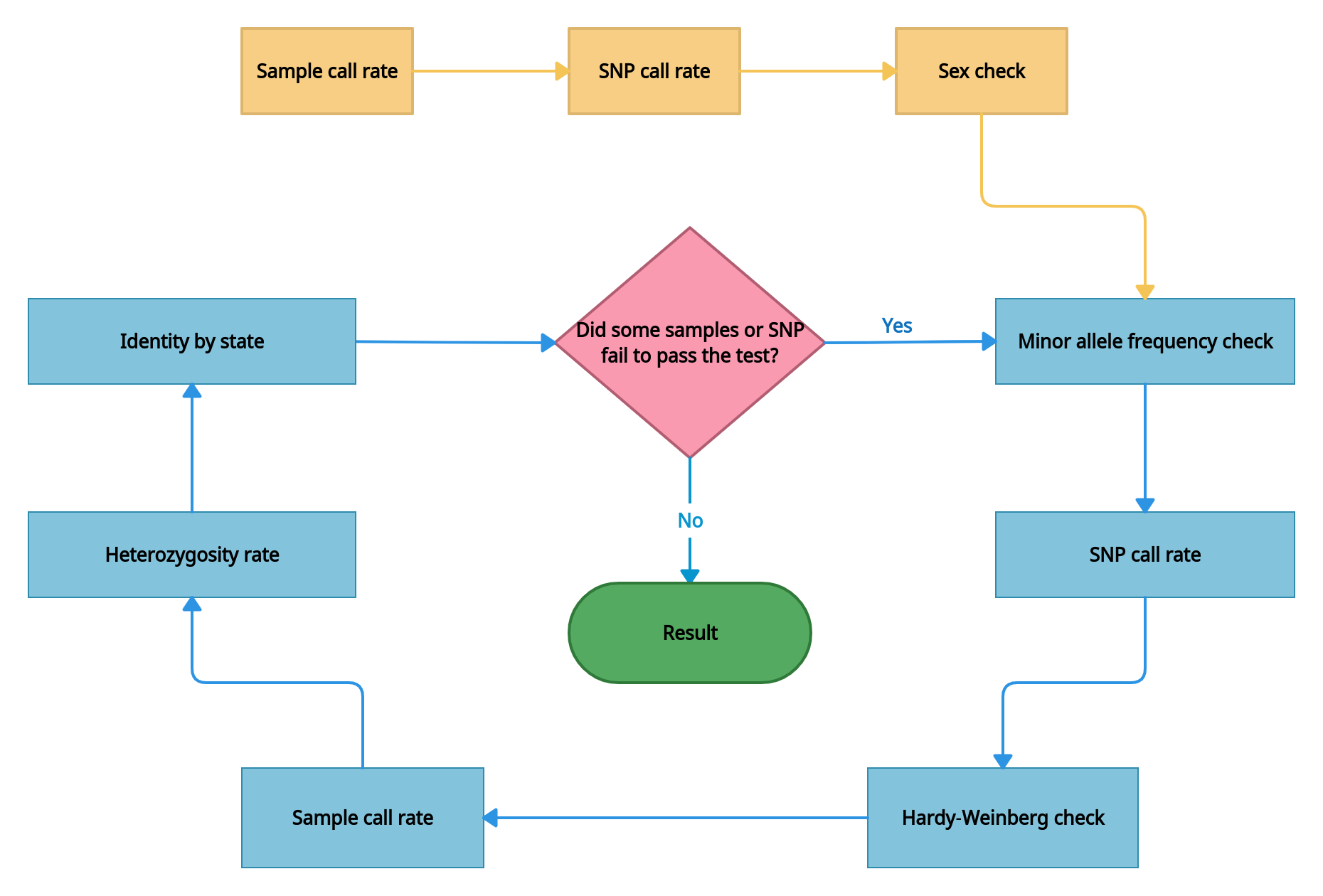
Checking the data for samples with extremely low call rate. Samples with high missing call rate are implications of poor DNA quality. They are removed from analysis. The sample call rate threshold is > 0.5.
Checking the data for SNPs with extremely low call rate. The missing call rate of SNP is the proportion of samples whose genotypes are not called for a given SNP. SNPs with a high missing genotype rate (generally, >5%) imply some problems with the genotyping process, so these SNPs are eliminated from analysis. The SNP call rate threshold is > 0.5.
Sex check and removing samples with wrong sex assigned. Sex check is based on estimation of X-linked SNPs heterozygosity. By default, X-chromosome inbreeding coefficient F estimates smaller than 0.2 yield female samples, and values larger than 0.8 yield male samples.
Minor allele frequency (MAF) check. SNPs with MAF less than 1% are excluded from subsequent analysis as current SNP-chips genotyping rare variants (i.e. a locus with MAF< 1%) is difficult and error-prone. Thus, very low-frequency alleles are likely to represent genotyping error and may result in spurious associations.
SNP filtration by call rate with a threshold > 0.98.
Hardy-Weinberg equilibrium (HWE) check. Under Hardy-Weinberg’s assumptions, allele and genotype frequencies can be estimated from one generation to the next. It is noted that departure from Hardy-Weinberg equilibrium can occur due to selection, population admixture, cryptic relatedness, genotyping error, and genuine genetic association. So it is beneficial to check whether the SNPs deviate from HWE for quality control.
Sample filtration by call rate with a threshold > 0.98.
Sample heterozygosity. The proportion of heterozygous genotypes across an sample's genome can detect several issues with genotyping, like sample contamination, inbreeding. Samples that deviate ± 3 SD (standard deviation) from the sample's mean heterozygosity are removed from the analysis.
Identity by state check. A high degree of relatedness between samples can also generate inflation of the association. To investigate the cryptic relatedness we calculate kinship matrix and filter samples with close relationships. Kinship coefficient is > 0.0925.
A file with a detailed description of the quality control task log can be downloaded in the "Result files" section in the "Quality Filter" task details ("Download QC log TXT").

Second check and filtering of variants and generation of a new PLINK 2 binary fileset set with filtered samples and SNPs using PLINK.
A file with a detailed description of this task log can be downloaded in the "Result files" section in the "Quality Filter" task details ("Download merge log TXT").
A file with SNPs removed from the analysis can be downloaded in the same section ("Download Skipped variants TXT"). For each SNP, the reason for removing and the QC iteration run number at which the removing occurred are indicated.
The full data quality control report can be opened in the same section ("Open QC report HTML").
A file with samples removed from the analysis can be downloaded in the same section ("Download Removed samples TXT"). For each sample, the reason for removing and the QC iteration run number at which the removing occurred are indicated.
Excluding SNPs that did not pass filtering from analysis using vcftools.
Compressing a file into a GZIP archive using bgzip. The resulting file can be downloaded in the "Result files" section in the "Quality Filter" task details ("Download Filtered VCF_GZ").
Indexing a file using tabix. The resulting index file can be downloaded in the same section ("Download Filtered VCF_TBI").

Imputation#

Imputation is a statistical method for reconstructing missing genetic data based on haplotype analysis in a reference set.

bcftools index creates an index for a VCF file.
Dividing variants by chromosomes for parallel imputation using bcftools view.
Beagle phases genotypes and imputes ungenotyped markers.
Concatenating the imputed variants, divided by chromosomes, into a single VCF file using bcftools concat.
bcftools index creates an index for a VCF file.
Comparison of the original file and the file obtained after imputation, and generating a file with unimputed variants using vcftools.
Compressing a file with unimputed variants into a GZIP archive using bgzip.
bcftools index creates an index for a file with unimputed variants.
bcftools filter includes only imputed sites for which DR2 (dosage R-squared) > 0.3.
bcftools index creates an index for a file with imputed and filtered variants.
Concatenating the unimputed variants and filtered imputed variants into a single VCF file using bcftools concat.
bcftools index creates an index for a merged file.
A file with a detailed description of the imputation task log can be downloaded in the "Result files" section in the "Imputation" task details ("Download Impute log TXT").
A file with unimputed and filtered imputed variants in VCF format can be downloaded in the same section ("Download Imputed VCF_GZ").
An index file for VCF file can be downloaded in the same section ("Download Imputed VCF_TBI").

Determining sex#

Regardless of the sequencing type, sex information is imputed from the X-chromosome homozygosity level data for all samples. The X-chromosome inbreeding coefficient F is calculated using the following formula:

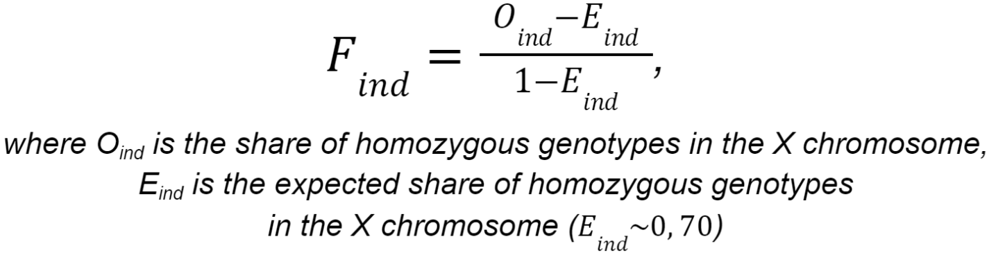
If F < 0.2, then the sex is determined as female. If F > 0.8, then the sex is determined as male. If 0.2 < F < 0.8, then the sex cannot be determined unambiguously.

The sex value determined from the genetic data is used when generating a report on polygenic traits. If this value does not match the patient's sex you specified, the value determined from the genetic data will be taken into account.

Polygenic risk scores calculation#

Polygenic risk scores calculation is launched after sample preprocessing steps has been successfully completed if the corresponding parameter is enabled.

1. Normalize multiallelic VCF#

Normalization of multiallelic VCF is a necessary step before calculating polygenic risk scores. bcftools norm left-aligns and normalizes indels; checks if reference alleles in the file match the reference; joins biallelic sites into multiallelic records. The resulting file with normalized variants is compressed into a GZIP archive using bgzip. You can download it in the "Result files" section in the "Normalize multiallelic VCF" task details ("Download VCF_GZ"). In addition, the file is indexed using tabix. The resulting index file can be downloaded in the same section ("Download VCF_TBI").

2. Polygenic risk scores calculation#

Polygenic risk scores calculation consists of applying a linear scoring to each sample using PLINK. Variants for which genotype information is missing for the site (genotype ./. etc.), variants without ID, or with mismatched allele codes are not taken into account in the analysis. The patient's genetic data must include the variants represented in the polygenic risk model, with the exception of a small proportion set by the threshold value. Polygenic risk scores calculation is considered possible if the user's genetic data contains at least 95% of all variants represented in the model.

The polygenic risk score (PRS) represents the total number of genetic variants (SNPs) that an individual has to assess their heritable risk of developing a particular phenotype. For each trait, the polygenic risk score is calculated using the following formula:

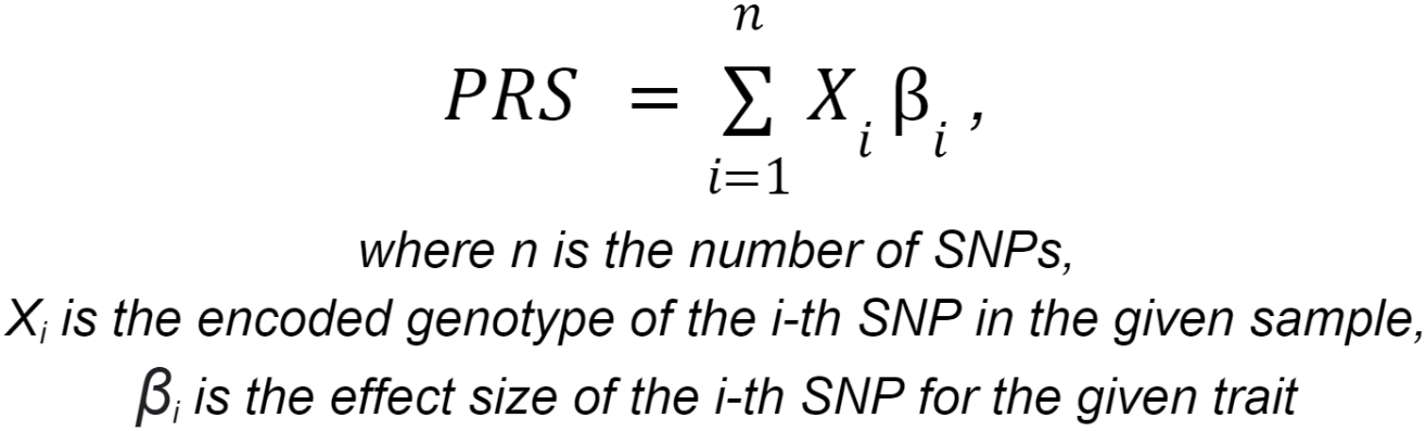
Genotypes are coded as follows: considering allele A as the effect allele and allele G as the ineffect allele, the numerical code for genotype AA is 2, genotype AG is 1, and genotype GG is 0.
The estimated effect sizes of SNPs are calculated based on genome-wide association study (GWAS) data, which match phenotypic traits with genomic variants in human populations.
The polygenic risk score reflects an individual's estimated genetic predisposition to the given trait and can be used as a predictor of that trait in a predictive model. In other words, the PRS estimates how likely an individual is to have the given trait based only on genetic data and without taking into account environmental factors.

The polygenic risk scores are calculated for the following traits:

Height
Weight
Body Mass Index (BMI)
Predisposition to being overweight
Predisposition to Prostate Cancer
Predisposition to Breast Cancer
Predisposition to Coronary Artery Disease
Predisposition to Inflammatory Bowel Disease
Predisposition to Type 2 diabetes
Predisposition to Colorectal Cancer

For each trait, three files are generated as a result, which can be downloaded in the "Result files" section in the "Polygenic risk scores calculation" task details:

A file with a detailed description of PRS calculation log ("Download [the trait name] Prs log TXT").
A file with the summary risk score for this sample ("Download [the trait name] Score TSV"). You can also open it in Google Sheets.
A file with a list of variant IDs used to calculate PRS ("Download [the trait name] Used Variants TSV"). You can also open it in Google Sheets.

Phenotypes prediction#

Phenotypes prediction (oligogenic risk calculation) is launched after sample preprocessing steps has been successfully completed if the corresponding parameter is enabled.

1. Normalize VCF#

First, VCF file is normalized using bcftools norm that left-aligns and normalizes indels; checks if reference alleles in the file match the reference; splits multiallelic sites into biallelic records; outputs only the first instance if a record is present multiple times. The resulting file is compressed into a GZIP archive using bgzip. You can download it in the "Result files" section in the "Normalize VCF" task details ("Download VCF_GZ"). In addition, the file is indexed using tabix. The resulting index file can be downloaded in the same section ("Download VCF_TBI").

2. Phenotypes prediction#

During the task execution, the following oligogenic risks are calculated:

Hair color: The probability is predicted by a model that uses Multinomial Logistic Regression. Hair color is determined by 22 polymorphisms, the model¹ predicts probabilities for 4 categories: black, brown, red, blond hair color. Hair shade is determined by 20 polymorphisms (intersecting with hair color), the model predicts probabilities for dark and light hair shade. The phenotype is predicted by combining the probabilities from both models.
Eyes color: The probability is predicted by a model that uses Multinomial Logistic Regression. Eyes color is determined by 6 polymorphisms, the model² predicts probabilities for three phenotypic traits: blue, green, brown eyes color.
Skin color: The probability is predicted by a model that uses Multinomial Logistic Regression. Skin color is determined by 36 polymorphisms. The skin phenotype is determined by the Fitzpatrick scale³. The model⁴ predicts probabilities for 5 phenotypic traits: very dark, dark, medium, fair, and very fair skin color.
Freckling: The probability is predicted by a model that uses Multinomial Logistic Regression. The model⁵ predicts the presence of freckles based on 14 predictors (one of which is sex). It predicts 3 types of freckling: severe, medium, and absence.
Lactose intolerance: The model is based on one polymorphism that completely associates with biochemically verified lactase non-persistence⁶. Secondly and thirdly, some polymorphisms are considered that may be responsible for the variability of this trait for some populations (Finnish⁶, East African⁷).
Bitter taste: The model is based on three polymorphisms giving rise to five haplotypes in the gene that encodes a member of the TAS2R bitter taste receptor family. These haplotypes completely explain the bimodal distribution of phenylthiocarbamide taste sensitivity⁸.
Blood type: The model is based on a haplotype consisting of 2 polymorphisms⁹.
Alcohol metabolism: The model is based on a single polymorphism, a substitution in which has been shown to result in the formation of a nearly inactive ALDH2 enzyme that no longer oxidizes acetaldehyde to acetate¹⁰. Having even one allele is fully protective against alcoholism. In fact, the protective effect of this polymorphism is the most widely replicated association of a specific gene with alcoholism¹¹. Another polymorphism that is frequently present in studies¹¹ is considered secondarily.
Earwax: The model is based on a single polymorphism in the ABCC11 gene¹² that contains instructions for a protein that specializes in moving fat into and out of the cells. People who have 1 or 2 copies of the C variant in the ABCC11 gene have more fat in their earwax, making it dark-colored and sticky. People who have two copies of the T variant have less fat in their earwax, making it dry, light-colored, and flaky.
Body odour: The model is based on a single polymorphism that is strongly associated with axillary osmidrosis¹³.
Pharmacokinetic: Prediction of risks of using certain drugs based on recommendations for the use of pharmacogenetic testing in clinical practice¹⁴.

Drug name	Marker	Risk score	Risk description and recommendations
Statins (Atorvastatin, Simvastatin, Fluvastatin, Rosuvastatin, Pravastatin)	1 SNP	0	"Wild type" genotype does not require statin dose adjustment.
		1	Associated with a high risk of myopathy, including rhabdomyolysis, when using simvastatin, atorvastatin, pravastatin or rosuvastatin. The maximum dose of statins allowed is 40 mg/day.
		2	Associated with a high risk of myopathy, including rhabdomyolysis, when using simvastatin, atorvastatin, pravastatin or rosuvastatin. The maximum dose of statins allowed is 20 mg/day.
Tacrolimus	1 SNP	0	Tacrolimus is well tolerated. There are no alleles that increase nephrotoxicity.
		1	Associated with the development of nephrotoxicity when tacrolimus is administered using the standard dosing. People with heterozygous genotype are more sensitive to tacrolimus than people with "wild type" homozygous genotype.
		2	Associated with the development of nephrotoxicity when tacrolimus is administered using the standard dosing. People with homozygous genotype are most sensitive to tacrolimus.
Azathioprine and 6-mercaptopurine	9 SNPs	1	Associated with a high risk of developing hematological toxicity in the first week of treatment with azathioprine or 6-mercaptopurine at standard doses. It is recommended to initiate treatment with azathioprine or 6-mercaptopurine at 50% of the standard dose.
Azathioprine and 6-mercaptopurine	9 SNPs	2	Associated with a high risk of developing hematological toxicity in the first week of treatment with azathioprine or 6-mercaptopurine at standard doses. It is recommended to initiate treatment with azathioprine or 6-mercaptopurine at 10% of the standard dose.
Abacavir	1 SNP	1	Associated with the development of hypersensitivity syndrome with the use of abacavir¹⁴. It is recommended to discontinue the use of abacavir.
Clopidogrel	2 SNPs	1	A weak antiplatelet effect of clopidogrel is noted due to the disruption of the formation of its active metabolite in the liver, which is the basis for genetically determined resistance to this drug. Patients with these allelic variants receiving clopidogrel have a higher risk of cardiovascular events compared to patients who do not carry these allelic variants.
Tamoxifen	7 SNPs and a deletion of the CYP2D6 gene	1	Associated with a slowdown in the formation of the active metabolite of tamoxifen in the liver and predicts low efficacy of tamoxifen in patients with postmenopausal estrogen-positive breast cancer.
Irinotecan	1 SNP	1	Associated with impaired biotransformation of the active metabolite of irinotecan SN-38, its accumulation in the body and a high risk of developing neutropenia and severe diarrhea.

Misophonia: The model is based on a single polymorphism that is significantly associated with the sensitivity to chewing sounds¹⁵.
Sleep movement: The model is based on a single polymorphism that is associated with restless legs syndrome and susceptibility to periodic limb movements in sleep¹⁶.
Photic sneeze reflex: The model is based on two polymorphisms that are associated with photic sneeze reflex¹⁷.
Sex: the result of the "Determining sex" task described above.

The resulting file with predicted phenotypes can be downloaded in the "Result files" section in the "Phenotypes prediction" task details ("Download Classifier results JSON").

After the "Phenotype prediction" stage, the analysis can proceed with report generation.